Sparse optical flow models
Severe weather conditions evolve fast, so it might be not enough to use NWP forecasts only to predict (especially local) rainfall rates correctly for an hour (or less) in advance.
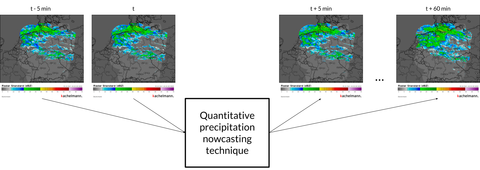
General idea of nowcasting is to use series of consecutive radar images for predicting the next ones with lead times up to 2 hours and time resolution from 5 to 20 minutes.
You can refer to the best review of nowcasting techniques and its classification by J. Wilson et. al. (1998)
Here we will briefly describe and implement the models from the Sparse group of the rainymotion library:
SparseSD model
Sparse model
The SparseSD model
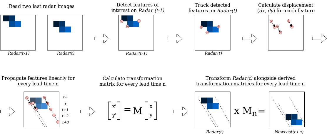
The implementation of the SparseSD model can be summarized as follows:
Identify features in a radar image at time t-1 using the Shi-Tomasi (Shi and Tomasi, 1994) corner detector;
Track these features at time t using the local Lukas-Kanade (Lukas and Kanade, 1981) optical flow algorithm;
Linearly extrapolate the features’ motion in order to predict the features’ locations at each lead time n;
Calculate the affine transformation matrix (Schneider and Eberly, 2003) for each lead time n based on the features’ locations at time t and t+n;
Warp the radar image at time t for each lead time n using the corresponding affine matrix, and linearly interpolate remaining discontinuities (Wolberg, 1990).
The SparseSD model usage example:
# import the model from the rainymotion library
from rainymotion.models import SparseSD

# initialize the model
model = SparseSD()

# upload data to the model instance
model.input_data = np.load("/path/to/data")

# run the model with default parameters
nowcast = model.run()
The Sparse model
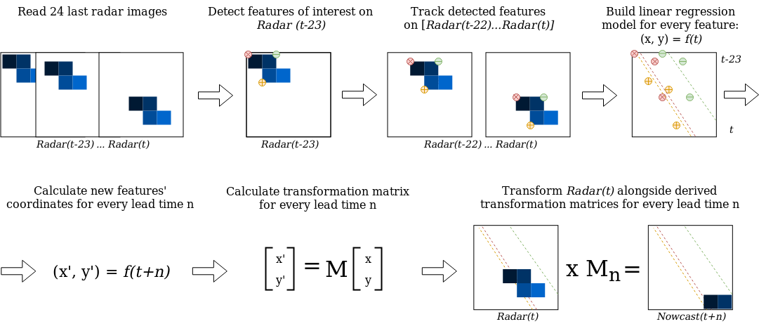
The implementation of the Sparse model can be summarized as follows:
Identify features on a radar image at time t-23 using the Shi-Tomasi (Shi and Tomasi, 1994) corner detector;
Track these features on radar images at the time from t-22 to t using the local Lukas-Kanade (Lukas and Kanade, 1981) optical flow algorithm;
Build linear regression models which independently parametrize changes in coordinates through time (from t-23 to t) for every successfully tracked feature;
Linearly extrapolate the features’ motion in order to predict the features’ locations at each lead time n;
Calculate the affine transformation matrix (Schneider and Eberly, 2003) for each lead time n based on the features’ locations at time t and t+n;
Warp the radar image at time t for each lead time n using the corresponding affine matrix, and linearly interpolate remaining discontinuities (Wolberg, 1990).
The Sparse model usage example:
# import the model from the rainymotion library
from rainymotion.models import Sparse

# initialize the model
model = Sparse()

# upload data to the model instance
model.input_data = np.load("/path/to/data")

# run the model with default parameters
nowcast = model.run()